Rebuilding a campus from public data
A 450 by 600 metre crop of the Illinois main quad, reconstructed as a gaussian splat and streamed to an ordinary browser. Every input is public domain or share-alike, and none of it is Google Street View. That exclusion is a design constraint rather than a disclaimer: it decides where the shape can come from, and therefore what the whole thing costs to build.
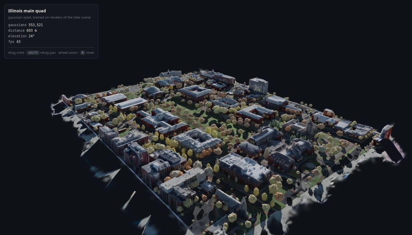
The question this project is a test of: how far can you rebuild a specific real place, to the point where somebody can move around inside it, using only data that anybody is allowed to download and republish? Everything else on this site asks what a model costs to run. This asks what a place costs to reconstruct, and the answer turns out to be set by two things that are not the GPU.
What it is made of
| source | what it supplies | licence |
|---|---|---|
| USGS 3DEP lidar, flown 2019, quality level 1 | all geometry. 20.02 points per m² measured over the crop, 2.5× the QL1 minimum | public domain |
| USDA NAIP orthoimagery, flown 2023, 30 cm | roof and ground colour, and the external reference for fidelity | public domain |
| OpenStreetMap, via Overpass | building names only, never geometry. 208 of 742 instances get one | ODbL |
Six lidar tiles, 537 MB, are the entire geometry input. The points arrive already classified, which deleted a planned stage of the pipeline: class 6 alone yields 742 building instances over the campus, so no footprint segmentation was needed and OpenStreetMap was demoted to labels. Ground is 27.2% of the crop, buildings 21.0%, vegetation 20.5%.
From that, a scene is built with materials, facades and tree species, rendered in Blender, and the splat is trained on those renders. So the model is a reconstruction of a measurement, not of a photograph, and the ordering matters for what it can be checked against.
Why Street View is out
Google's Geo Guidelines forbid downloading Street View imagery for offline use, stitching it, tracing information from it, running applications that extract information from it, and screenshotting it, and then say that these restrictions apply to all academic, nonprofit and commercial projects. There is a research channel, but it covers 114,000 panoramas in New York City and Pittsburgh and nothing else.
So the line drawn here is: looking at Street View in a browser to form a judgement is unrestricted and useful. Putting it in a figure, or computing anything from it, is not done, including in side-by-side comparisons.
This is the constraint that shapes the pipeline. With no ground-level photography of the site, shape has to come from an airborne survey and colour from a nadir photograph, which is also why facades are the part with no colour source yet. Every other decision below follows from it.
Where the density came from
The first whole-scene model was too thin to stand in: 549,220 gaussians over the crop, mean spacing 59 cm. The obvious lever runs out of road. Measured on one patch, three settings of the densification gradient threshold:
| densify threshold | gaussians | spacing |
|---|---|---|
| 0.0002 (reference) | 1× | 10.5 cm |
| 0.0001 | 2.2× | 7.5 cm |
| 0.00005 | 5.1× | 6.6 cm |
Five times the gaussians bought 37% finer spacing. What worked instead was cutting the scene into twenty pieces, for three reasons.
Memory forced it. The trainer holds every training image as a float32 tensor plus an all-ones alpha mask, 30.7 MB per view, so the 6,202-view set is 190 GB of host RAM on a machine with 62. Supervision explains most of the gain. Thirty thousand iterations over 6,202 views is 4.8 passes per view; a chunk of 553 views gets 54. And initialisation turned out to be the whole story. A chunk starts from all the lidar inside it, so twenty chunks begin from 11.6 M measured points where the whole crop had been sampled down to 400,000.
Four arms on one chunk, each changing one thing from the run before it, settled which of those mattered:
| arm | what changed | gaussians kept | spacing | train PSNR |
|---|---|---|---|---|
| A | reference settings | 125,228 | 50.4 cm | 28.01 |
| B | lower split threshold | 173,094 | 42.8 cm | 28.75 |
| C | three densification flags at once | 329,231 | 31.1 cm | 24.74 |
| D | denser initialisation, reference flags | 228,684 | 37.3 cm | 29.05 |
Arm C has the most gaussians and the worst reconstruction. It trained 2,634,882 of them and only 12.5% ended above an opacity of 0.1, losing 3.3 dB to spend the budget on near-transparent ones. Count is not the objective and it is not even a proxy for it. Arm D touched nothing but the starting point and beat every arm that tuned the optimiser, and the growth factors say why: A grew its initial points by 1.36×, D by 1.09×. The denser the start, the less densification does.
So the density control is the initialisation spacing, and the limit is not the card. At 7 cm initialisation a 16 GB card still had 6 GB spare and had only halved its rate. The stop is the data: the render rig's median ground sample distance is 3.5 cm, and below about twice that the optimiser is inventing detail rather than reconstructing it. Production sits on that line, at 7 cm on walls, 12 cm on roofs and canopy, 20 cm on ground.
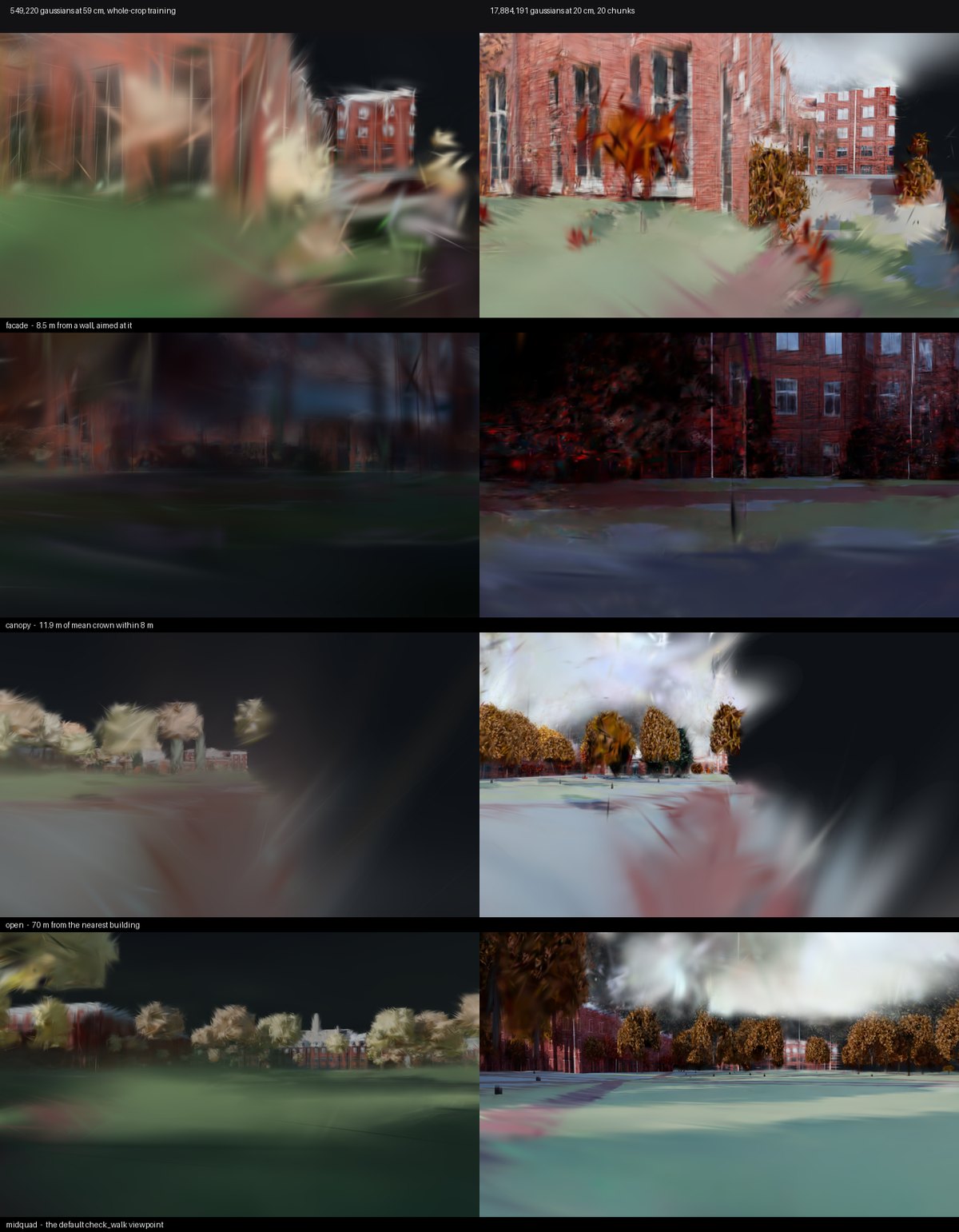
The twenty chunks were trained across two workstations by taking every nth chunk on each, with no coordination beyond a copy at the end. The same split was used for the render pass: 6.6 seconds a frame on one machine and 12.6 on the other, so a 2 to 1 division of the 6,202 views finishes both at once, about 7.5 hours of wall clock for 14 hours of work.
The constant everything was linear in
Every size in the plan, tile counts, level spacings, payload, is linear in one number: how large a gaussian may be on screen before the picture stops being of a place and starts being of gaussians. It had been 2.5 pixels because somebody had to write something down, and the budget moves by a factor of ten between 3 and 10. So it was measured, by training two splats of one patch and rendering both at eleven distances against Blender renders of the same poses.
τ is about 5 pixels, not 2.5, which makes every gaussian count in the plan four times too large, since the count goes as one over its square. And the measurement said something the placeholder never could: the failure past that point is not graceful blur but collapse. At three metres the model has lost more than three quarters of the truth at the largest scale in the frame. It has lost the picture, not its detail.
The first estimator was the wrong question and its own goodness of fit said so. It tried to fit the Gaussian blur that takes the truth onto the splat, on the theory that the answer is a length. A splat at three metres is not a blurred wall, it is a streaky ghost of one, and a blur model fits almost nothing. Before that was clear, the fit needed guards of its own: a 2 pixel displacement with perfect sharpness fitted as 1.83 pixels of blur, and a half-black frame ran to the top of the sigma grid and returned 24 pixels, reported as 5.66 metres of blur without comment. The replacement measure reads the ratio of the two radially averaged spectra at the frequency where it falls through a half, and was validated against known low passes of 2.7, 5.3 and 10.7 pixels, returning 2.7, 5.3 and 10.6.
That measurement is load-bearing rather than academic, because the tile manifest carries each level's spacing and the measured τ. A viewer picks a level by arithmetic, spacing times focal length over τ, rather than by a magic number.
Getting it into a browser
The model is cut into 285 tiles of 32 metres, square in plan and full height, at six levels of detail, streamed by distance: 1.07 GB on disk. A level is a decimation on a grid rather than a random sample, because dropping gaussians at random thins the places that were already thin and leaves holes a viewer reads as sky through a wall.
What ships is that ladder with its two finest levels left off and the remainder re-indexed: the same 285 tiles, four levels, 3,936,948 gaussians at the base, 167 MB, which fits inside a 1 GB static hosting limit and makes the whole hosting question go away. An opening view is 21.4 MB and zooming all the way in tops out at 66 MB.
Three of the bugs found on the way were budget bugs rather than rendering bugs, and all three cost bandwidth silently. The streamer was fetching 188 MB to draw 70, so 63% of every visit was downloaded and discarded; capping the transfer at 1.6× what the budget can draw brought it to 112.6 MB with the picture unchanged, at a correlation of 0.986 against an offscreen render. The tile heap was capped at 200 against the 285 the scene can show, so the page threw away tiles it was still looking at and fetched them straight back, about 110 tiles and 167 MB a minute from a camera that was not moving. And past 108 metres nothing was drawn at all, because a budget spent nearest-first never reaches the far side.
One useful negative: building a coarse ladder from scratch with a coarser base spacing came out at 611 MB instead of 167, because the base level is never decimated. Re-indexing the ladder that already exists is exact and needs no rebuild.
What is not fixed
The near field. Standing on the grass, the model is a haze rather than a place, and the measurement says more gaussians will not fix it. A 20 cm disc lying flat, seen from eye height ten metres away, is 20 cm wide on screen and 3 cm tall, so a ray along the grass composites hundreds of them, and halving the spacing doubles how many it passes through. This is why the page opens from above and the walk is behind a flag. The two routes scoped for it both replace gaussians with a surface where a surface belongs, rather than adding more.
Facades have no colour source. A nadir photograph holds no wall information. The share-alike street-level panoramas that would supply it are registered to about 3.76 metres of GPS residual where facade projection needs sub-metre, so that registration has to be solved first.
The roofs are white, and it is not a rendering fault. Roof gaussians average 0.522 brightness against 0.398 for ground and 0.310 for walls, and 28% of them are near-white and desaturated against 1 to 6% everywhere else. Roof texture is sharpened from the aerial photograph rather than repainted, a pale flat roof at midday is already near the top of that exposure, and the sky then lights the one surface facing the whole dome. The splat learned it faithfully. No viewer change reaches it.
The lidar is 2019 and the photography is 2023, so anything built or demolished in between is in one and not the other, and no check has been run for how much of the campus that affects.
The viewer is here, with its sources and method beside it. The companion note on this cluster is what a finished second of generated film costs.